Over recent years, data scientists and analysts are using ggplot2 to visualise their data. ggplot2 is able to deliver beautiful graphics for its users in a reproducible and customisable way. The idea behind the ggplot2 is a system based on the Grammar of Graphics. The task to produce a graph is divided into semantic components such as scales and layers. The ggplot2 package, created by Hadley Wickham, in 2005 takes care of the details of plotting when the data and aesthetics information is provided. We will have a tutorial on how to use ggplot2.

How to Use ggplot2

For this tutorial, we will use the dataset: gini coefficient (gini index) by country from the World Bank estimation. The information can be found in our dataset section at: https://wordpress.com/block-editor/post/ospinaforerolab.home.blog/434. At this page you will find the original dataset and the Rscript for the data transformation. After you run the data transformation:

Install ggplot2 Package in Rstudio

To use the ggplot2, we will need to install the package in Rstudio. Use the following code:

install.packages("ggplot2")

Load package into current project:

library("ggplot2")

Basic Arguments in ggplot

• data argument specify the dataset we are going to use in the plotting. It is required for ggplot function to work.

ggplot(data = bric_data)

• aes is an argument cotains the aesthetics information. It can specify the x, y axes.

aes(x = Country.Name, y = gini)

• Combine data + aes in ggplot function.

ggplot(data = bric_data, aes(x = Country.Name, y = gini))

Geom Function

The geom function adds a layer to a graph. Each geom function returns a layer. The geom is commonly used to represent the data points and provide additional aesthetics properties to reperesent variables. In coding, geom function will be added after ggplot function. This is done by using the + sign:

ggplot(data = bric_data, aes(x = Country.Name, y = gini)) + geom_col( )

Here is a list of frequent used geom_function and their usages:

Inside the geom function, it also allow a stats to offer an alternaitve way to build a layer. Additional information regarding the geom_function, specific arguments, and stats can be found at https://ggplot2.tidyverse.org/. The cheatsheet can be found at https://github.com/rstudio/cheatsheets/blob/master/data-visualization-2.1.pdf.

Scales

The scale functions connect the data values to their visual representation in the plot. The Scale functions can be used to add filled colour, change the location scale, shape of the visual representations, and size of the visual representations.

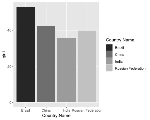
If we want to fill the bar chart with gradient colour, for example, we can use this grey colour fill:

ggplot(data = bric_data, aes(x = Country.Name, y = gini)) + 
  geom_col(aes(fill = Country.Name)) + 
  scale_fill_grey(start = 0.2, end = 0.8)

We will need to declare the values used for fill. aes(fill = Country.Name)

Coordinate System

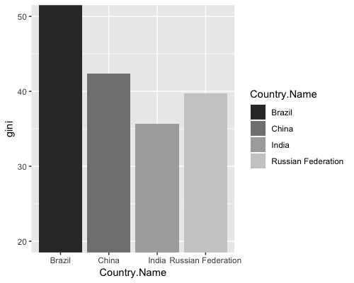
Coordinate function will give us the control to the coordinate and grid lines of the graph. Using a cartesian coordinate system for example, the code will be:

ggplot(data = bric_data, aes(x = Country.Name, y = gini)) + 
  geom_col(aes(fill = Country.Name)) + 
  scale_fill_grey(start = 0.2, end = 0.8) +
  coord_cartesian(ylim=c(20,50))

Now the grid lines for y-values will start at 20 and end at 50.

Themes

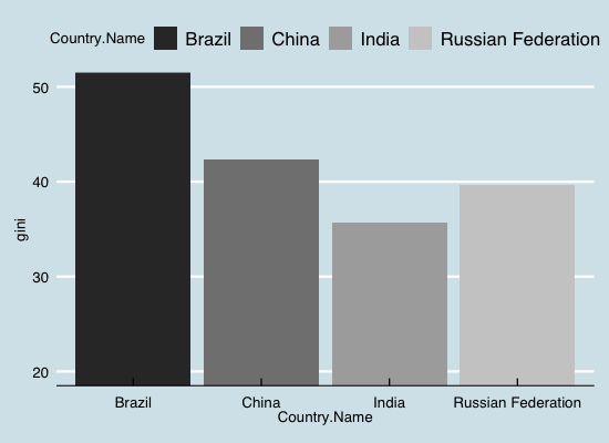
Themes function will allow us to import themes for our graph. We can add the economist theme (from ggtheme package, you will need to install and load ggtheme package) to our bar chart:

ggplot(data = bric_data, aes(x = Country.Name, y = gini)) + 
  geom_col(aes(fill = Country.Name)) + 
  scale_fill_grey(start = 0.2, end = 0.8) +
  coord_cartesian(ylim=c(20,50)) + 
  theme_economist()

More information on ggplot2‘s themes can be found at: https://www.datanovia.com/en/blog/ggplot-themes-gallery/

Labels

With the label function, we can change labels, title, subtitle, and caption. We can use this to change our bar chart’s labels:

ggplot(data = bric_data, aes(x = Country.Name, y = gini)) + 
  geom_col(aes(fill = Country.Name)) + 
  scale_fill_grey(start = 0.2, end = 0.8) +
  coord_cartesian(ylim=c(20,50)) + 
  theme_economist() + 
  labs(x = "Country Name", y = "Gini Coefficient", 
       title = "BRIC Countries' Gini Coeficient",
       subtitle = "at 2011", 
       caption = "Data From: World Bank")

Apply the Knowledge

Line graph: Gini Coeficient Across 9 Countries from 2004 to 2015

It is time we apply the knowledge to create another graph. This time we will use the melted_data1 and plot a line graph. We will also try out the color_brewer in the geom function.

ggplot(data = melted_data1, aes(x = year, y = value, group = Country.Name, color = Country.Name)) + 
  geom_line() +
  scale_color_brewer(type = "seq", palette = 16) +
  coord_cartesian(ylim = c(20,60)) +
  labs(x = "Year", y = "Gini Coefficient",
       title = "Gini Coefficient of 9 Countries",
       subtitle = "Time Series Data From 2004 - 2015",
       caption = "Data From: World Bank")

Reference

[^Urban]: Why The Urban Institute Visualizes Data with ggplot2, Avaliable at:https://medium.com/@urban_institute/why-the-urban-institute-visualizes-data-with-ggplot2-46d8cfc7ee67

[^BBC]: How the BBC Visual and Data Journalism team works with graphics in R, Avaliable at:https://medium.com/bbc-visual-and-data-journalism/how-the-bbc-visual-and-data-journalism-team-works-with-graphics-in-r-ed0b35693535