

It is a common issue to handle missing values in data preparation step before analysis. In R, missing values are represented by NA, and there are abundant NA-related functions in R to deal with NA values.
Since we would like to cluster the SDG indicators later, it is highly recommended to construct a filtering function to guarantee there are no NA values in filtered data set before applying clustering methods to. In this blog, a multiparameter filtering function (named as “format()”) will be introduced. Also, all auxiliary functions used in “format()” and any parameters introduced in “format()” will be explained. In the end, the filtering results will be illustrated as histograms of indicators over goals and targets, comparing with the unfiltered distributions.
However, this function is data-sensitive, so it could only be applied to data sets directly derived from World Bank Database of SDG indicators (https://databank.worldbank.org/reports.aspx?source=sustainable-development-goals-(sdgs)), this database includes observations of 375 indicators from 1990 to 2018 in 263 countries in total. Once downloaded, the data will be dispatched in a single .csv format file. Moreover, we also require an indicator list, which lists the goal, target and series code of each indicator.
In the main function, there are three filters. First one will remove indicators with few distinct values; second one will delete indicators with high NA value ratio; third one will intercept a time window to minimize the NA value ratio.

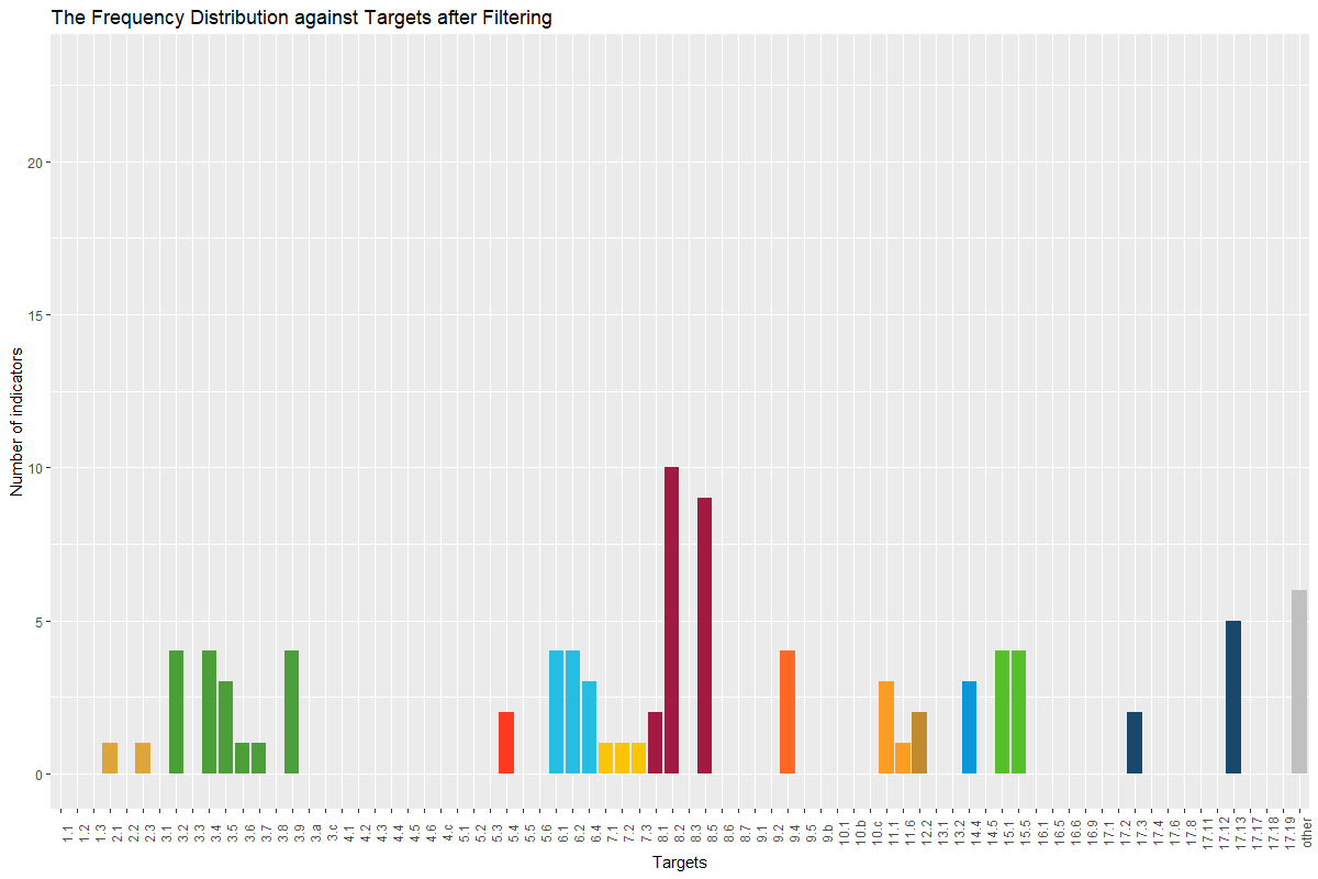
If we load the data of all 263 countries over 375 indicators from 1990 to 2016, and choose the minimum number of distinct values is 10, the maximum NA ratio is 30%, then 90 indicators will be preserved after three filters. And the distribution of these 90 indicators in goals and targets are shown below:


Following are all the codes and auxiliary functions used to form the filtering function. There will be a brief explanation before codes for each function, which will precisely define the parameters and output of this function and introduce what it does. In the end, the codes to form two visualization functions will be displayed as well.
Auxiliary Functions
# This function loads the file containing data then read it into R as a ‘data.frame’ data
# before use, replace the "_your_file_path_of_data_set_" .with your data file saved path
# Parameters:
###  filename (string) : the whole filename inclusive.csv
# Returns:
###  myData (data.frame): the data in the file
read.data <- function(fileName){
    fileName <- readline(prompt="Enter the file's name here:")
    filePath <- paste("_your_file_path_of_data_set_", fileName, sep="")
    myData <- fread(file=goalListPath, header=TRUE, sep=",")
    myData <- head(myData, -5)
    colnames(myData)[5:33] <- c(1990:2018)
    myData <- as.data.frame(myData)
    return(myData)
    }

# This function returns the list of data with all outliers removed
# Parameters:
###  x (vector): a list of numeric values
# Returns:
###  y (vector): the list values exclusive outliers
remove.outliers <- function(x){
    qnt <- summary(x)
    H <- 1.5 * (qnt[5]-qnt[2])
    y <- x[(qnt[2]-H) < x & x < (qnt[5]+H)]
    return(y)
}

# This function returns the indicator list with removing indicators whose ‘code’ is in the ‘list’
# Parameters:
###  data (data.frame): the raw indicator list
###  list (vector): the list of indicators’ codes to delete
# Returns:
###  data (data.frame): the indicator list after conditionally removing
indicator.remove <- function(data, list){
    for (x in list){
         data <- data[!(data$`Code`==x),]
    }
    return(data)
}
Filtering by Number of Distinct Values – 1st filter
# This function returns a data.frame indicating the number of distinct values for each indicator in every country
# Parameters:
### data(data.frame): the raw data
# Returns:
### indNumValue(data.frame): a data frame with three columns as ‘country name’, ’series code’ and number of distinct values corresponding to this indicator in this country
indicator.number <- function(data){
    i <- 1
    n <- NROW(data)
    m <- NCOL(data)
    seriesNum <- c()
    while (i <= n){
        valueList <- na.omit(as.numeric(data[i,5:m]))
        numValue <- length(unique(valueList))
        seriesNum <- c(seriesNum, numValue)
        i <- i + 1
    }
    indNumValue <- cbind(data[,c(1,4)],'Number of Distinct Values'=seriesNum)
    return(indNumValue)
 }

# This function returns a list of ‘series code’ of indicators whose minimum value of numbers of distince values over all countries (with outliers removed) is smaller than ‘cv’
# Parameters:
### data (data.frame): the data frame of number of distinct values in every indicators obtained from former function
### cv (string): the critical value of minimum number of distinct values
# Returns:
### seriesCode (vector): a list of indicators’ codes to delete
remove.ind1 <- function(data,cv){
    seriesCode <- c()
    for (x in data) {
        list <- x[,3]
        list <- as.numeric(as.matrix(list))
        minValue <- min(remove.outliers(list))
        if (minValue < cv){
            seriesCode <- c(seriesCode, x[1,2])
        }
    }
    return(seriesCode)
}

# This function returns the data.frame with removing indicators whose minimum value of number of distinct values is smaller than ‘n’
# Parameters:
###  data (data.frame): the data frame of number of distinct values in every indicators obtained from former function
###  Data (data.frame): the raw data
###  n (string): the critical value of number of distinct values
# Returns:
###  Data (data.frame): the data after conditionally removing rows
###  series1 (vector): the 1st list of indicators’ codes to delete
remove.data1 <- function(data, Data, n){
    dataNa <- data[!data$`Number of Distinct Value`==0,]
    dataInd <- split(dataNa, dataNa$`Series Code`)
    series1 <- remove.ind1(dataInd,cv=n)
    for (x in series1) {
        Data <- Data[!Data$`Series Code`==x,]
    }
    return(list(Data, series1))
}
Filtering by Indicators-NA Ratio – 2nd filter
# This function returns a list of NA ratio for each indicator in every country
# Parameters:
### data (data.frame): the data after 1st filter
# Returns:
### series1 (vector): a list of numeric values which are the NA ratio in years for each indicator
series.na1 <- function(data){
    i <- 1
    n <- NROW(data)
    m <- NCOL(data)
    series1 <- c()
    while (i <= n){
        naRatio <- sum(is.na(as.numeric(data[i,5:m])))/(m-4)
        series1 <- c(series1, naRatio)
        i <- i + 1
    }
    return(series1)
}

# This function returns a data.frame indicating the NA ratio in years for each indicator in every country
# Parameters:
### data (data.frame): the data after 1st filter
# Returns:
### indicatorNA (data.frame): a data frame with three columns as ‘country name’, ’series code’ and NA ratio in years corresponding to this indicator in this country
indicator.na <- function(data){
    seriesNA <- series.na1(data)
    indicatorNA <- data[,c(1,4)]
    indicatorNA <- cbind(indicatorNA, "NA Ratio"=seriesNA)
    return(indicatorNA)
}

# This function returns a list of ‘series code’ of indicators whose maximum value of NA ratio over all countries (with outliers removed) smaller than ‘r’
# Parameters:
### data (data.frame): the data frame of NA ratio in every indicators obtained from former function
### r (string): the critical value of maximum value of NA ratio
# Returns:
### seriesCode (vector): a list of indicators’ codes to delete
remove.ind2 <- function(data,r){
    seriesCode <- c()
    for (x in data) {
        list <- x[,3]
        list <- as.numeric(as.matrix(list))
        maxValue <- max(remove.outliers(list))
        if (maxValue > r){
            seriesCode <- c(seriesCode, x[1,2])
        }
    }
    return(seriesCode)
}

# This function returns the data.frame with removing indicators whose maximum value of NA ratio is smaller than ‘n’
# Parameters:
###  data (data.frame): the data frame of NA ratio in every indicators obtained from former function
###  Data (data.frame): the data obtained from the former filter
###  n (string): the critical value of NA ratio
# Returns:
###  Data (data.frame): the data after conditionally removing rows
###  series2 (vector): the 2nd list of indicators’ codes to delete
remove.data2 <- function(data, Data, n){
    dataInd <- split(data,data$`Series Code`)
    series2 <- remove.ind2(dataInd, r=n)
    for (x in series2) {
        Data <- Data[!Data$`Series Code`==x,]
    }
    return(list(Data, series2))
}
Filtering by Year-NA Ratio – 3rd filter
# This function returns a list of NA ratio over indicators for each year in every country
# Parameters:
### data (data.frame): the data after 1st and 2nd filters
# Returns:
### series2 (vector): a list of numeric values which are the NA ratio in indicators for each year
series.na2 <- function(data){
    i <- 5
    n <- NROW(data)
    m <- NCOL(data)
    series2 <- c()
    while (i <= m){
        naRatio <-sum(is.na(as.numeric(t(data[1:n,i]))))/n
        series2 <- c(series2, naRatio)
        i <- i + 1
    }
    return(series2)
}

# This function returns a data.frame indicating the NA ratio in indicators for each year in every country
# Parameters:
### data(data.frame): the data after 1st and 2nd filters
# Returns:
### yearNA (data.frame): a data frame with three columns as ‘country name’, ’series code’ and NA ratio in indicators corresponding to this year in this country
year.na <- function(data){
    countryList <- data$`Country Name`
    countryList <- countryList[!duplicated(countryList)]

    dataCountry <- split(data, data$`Country Name`)
    yearNAseries <- c()
    n <- length(countryList)
    m <- NCOL(dataCountry[[1]])
    yearName <- colnames(dataCountry[[1]])[5:m]
    for (x in dataCountry) {
        series2 <- series.na2(x)
        yearNAseries <- c(yearNAseries, series2)
    }
    yearNA <- data.frame(matrix(, nrow = n*(m-4), ncol = 0))
    yearNA <- cbind(yearNA, "Country" = rep(countryList,each=(m-4)),
                    "Year" = rep(yearName, times=n),
                    "NA Ratio" = yearNAseries
                    )
    return(yearNA)
}
Main Filtering Function
format.data <- function(write=FALSE){
    myData <- read.data()

    indNum <- indicator.number(myData)
    t <- readline(prompt="Enter the minimum number of distince values:")
    x <- remove.data1(indNum, myData, n = as.numeric(t))
    myData1 <- x[[1]]
    series1 <- x[[2]]

    indNA <- indicator.na(myData1)
    r <- readline(prompt="Enter the maximum value of NA ratio:")
    y <- remove.data2(indNA, myData1, n = as.numeric(r))
    myData2 <- y[[1]]
    series2 <- y[[2]]

    year1 <- readline(prompt="Enter the start year of time windows:")
    year2 <- readline(prompt="Enter the end year of time windows:")
    year1 <- as.numeric(year1)-1985
    year2 <- as.numeric(year2)-1985
    myData3 <- subset(myData2, select=c(1:4,year1:year2))

    IndNum <- indicator.number(myData3)
    IndNA <- indicator.na(myData3)
    YearNA <- year.na(myData3)

    indicatorList <- fread(file = "_your_file_path_of_indicator_list_",
                           header=TRUE, sep=",")
    seriesList <- c(series1, series2)
    IndList <- indicator.remove(indicatorList, seriesList)

    if (write) {
        fileName <- readline(prompt="Enter the name of indicator list:")
        write.csv(IndList, file=paste("_your_file_path_of_output_", fileName, sep=""), row.names = FALSE)

        fileName <- readline(prompt="Enter file name of number of distinct values against indicators:")
        write.csv(IndNum, file=paste("_your_file_path_of_output_", fileName, sep=""), row.names = FALSE)

        fileName <- readline(prompt="Enter file name of NA ratio against indicators:")
        write.csv(IndNA, file=paste("_your_file_path_of_output_", fileName, sep=""), row.names = FALSE)

        fileName <- readline(prompt="Enter file name of NA ratio against years:")
        write.csv(YearNA, file=paste("_your_file_path_of_output_", fileName, sep=""), row.names = FALSE)

        IndNumBoxplot <- ggplot(IndNum,aes(x=`Series Code`,
                                           y=`Number of Distinct Value`, group=`Series Code`))+
            geom_boxplot(fill = '#A4A4A4',color = 'black',
                         outlier.color ='darkblue',outlier.size = 0.2)+
            ggtitle("Number of Distinct Values with respect to Indicators") +
            xlab("Series Code of Indicators") +
            ylab("Number of Distinct Value") +
            theme(plot.title = element_text(hjust=0.5, size=20, face="bold"),
                  axis.title.x = element_text(size=15, face="bold"),
                  axis.title.y = element_text(size=15, face="bold"),
                  axis.text.x = element_text(angle=90))

        IndNABoxplot <- ggplot(IndNA, aes(x=`Series Code`, y=`NA Ratio`,
                                           group=`Series Code`)) +
            geom_boxplot(fill='#A4A4A4',color='black',
                         outlier.color ='darkblue',outlier.size = 0.2) +
            ggtitle("NA Ratio of Country Data with respect to Indicators") +
            xlab("Series Code of Indicators") +
            ylab("NA Ratio")+
            theme(plot.title = element_text(hjust=0.5, size=20, face="bold"),
                  axis.title.x = element_text(size=15, face="bold"),
                  axis.title.y = element_text(size=15, face="bold"),
                  axis.text.x = element_text(angle=90))

        YearNABoxplot <- ggplot(YearNA, aes(x=`Year`, y=`NA Ratio`, group=`Year`)) +
            geom_boxplot(fill = '#A4A4A4',color = 'black',
                         outlier.color ='darkblue',outlier.size = 0.2) +
            ggtitle("NA Ratio of Country Data with respect to Years") +
            xlab("Year") +
            ylab("NA Ratio") +
            theme(plot.title = element_text(hjust=0.5, size=15, face="bold"),
                  axis.title.x = element_text(size=10, face="bold"),
                  axis.title.y = element_text(size=10, face="bold"),
                  axis.text.x = element_text(angle=90))

        ggsave("Number_of_Distinct_Values.png", IndNumBoxplot, device="png",
               path="_your_file_path_of_output_plot_", scale=2, width=15, height=8, units="cm")
        ggsave("NA_Ratio_of_Indicators.png", IndNABoxplot, device="png",
               path="_your_file_path_of_output_plot_", scale=2, width=15, height=8, units="cm")
        ggsave("NA_Ratio_of_Years.png", YearNABoxplot, device="png",
               path="_your_file_path_of_output_plot_", scale=2, width=9, height=6, units="cm")
    }
    return(list(myData3, IndList, IndNum, IndNA, YearNA))
}
Visualization of Indicators’ Distribution
# This function returns a histogram of indicators distribution over goals
# Parameters:
### indCode(vector): a list of character values(series codes of left indicators)
### fileName(string): the filename of indicator list
# Returns:
# IndFreqGoal(boxplot): the histogram of indicators' frequency over goals
ind.freq.goal <- function(indCode) {
    fileName <- readline(prompt = "Enter the file name of indicator list here:")
    indList <- fread(file=paste("_your_file_path_of_indicator_list",fileName, sep=""), header=TRUE,sep=",")
    IndList <- indList[indList$'Code' %in% indCode,]
    IndGoal <-IndList[,1]
    goalFreq <- data.frame(matrix(,nrow=18,ncol=0))
    freqSeries <- c()
    for (i in c(1:18)){
        indFreq <- sum(IndGoal==i)
        freqSeries <- c(freqSeries, indFreq)
    }
    goalFreq <- cbind(goalFreq,'Goal'=c(1:18),'Freq'=freqSeries)
    goalFreq$Goal <- as.numeric(as.character(goalFreq$Goal))
    goalFreq <- goalFreq[order(goalFreq$Goal),]
    goalFreq$Goal <- factor(goalFreq$Goal, levels=c(1:17,'others'))
    goalFreq[18,1] <- 'others'
    IndFreqGoal <- ggplot(goalFreq, aes(x=Goal, y=Freq, fill=Goal))+
        geom_bar(stat="identity", width=0.7)+
        scale_fill_manual(values = c("#E5243B", "#DDA63A", "#4C9F38",
                                     "#C5192D", "#FF3A21", "#26BDE2",
                                     "#FCC30B", "#A21942", "#FD6925",
                                     "#DD1367", "#FD9D24", "#BF8B2E",
                                     "#3F7E44", "#0A97D9", "#56C02B",
                                     "#00689D", "#19486A", "#C0C0C0"))+
        ggtitle("The Frequency Distribution against Goals after Filtering")+
        xlab("Goals")+ylab("Number of indicators")+
        scale_y_continuous(breaks = seq(0,90, by=20))+
        theme(legend.position="none")
    return(IndFreqGoal)
}

# This function returns a histogram of indicators distribution over targets
# Parameters:
### indCode(vector): a list of character values(series codes of left indicators)
### fileName(string): the filename of indicator list
# Returns:
# IndFreqGoal(boxplot): the histogram of indicators' frequency over targets
ind.freq.target <- function(indCode) {
    fileName <- readline(prompt = "Enter the file name of indicator list here:")
    indList <- fread(file=paste("_your_file_path_of_indicator_list",fileName, sep=""), header=TRUE,sep=",")
    IndList <- indList[indList$'Code' %in% indCode,]
    IndTarget <-IndList[,2]
    targetList <- c(1.1,1.2,1.3,2.1,2.2,2.3,3.1,3.2,3.3,3.4,3.5,3.6,3.7,3.8,3.9,"3.a","3.c",
                    4.1,4.2,4.3,4.4,4.5,4.6,"4.c",5.1,5.2,5.3,5.4,5.5,5.6,6.1,6.2,6.4,7.1,7.2,
                    7.3,8.1,8.2,8.3,8.5,8.6,8.7,9.1,9.2,9.4,9.5,"9.b",10.1,"10.b","10.c",11.1,
                    11.6,12.2,13.1,13.2,14.4,14.5,15.1,15.5,16.1,16.5,16.6,16.9,17.1,17.2,17.3,
                    17.4,17.6,17.8,17.11,17.12,17.13,17.17,17.18,17.19,18)
    targetFreq <- data.frame(matrix(,nrow=76,ncol=0))
    freqSeries <- c()
    for (x in targetList){
        indFreq <- sum(IndTarget==x)
        freqSeries <- c(freqSeries, indFreq)
    }
    targetFreq <- cbind(targetFreq,'Target'=targetList,'Freq'=freqSeries)
    targetFreq$Target <- factor(targetFreq$Target, levels=c(targetList[1:75],'others'))
    targetFreq[76,1] <- 'others'
    IndFreqTarget <- ggplot(targetFreq, aes(x=Target, y=Freq, fill=Target))+
        geom_bar(stat="identity", width=0.7)+
        scale_fill_manual(values = rep(c("#E5243B", "#DDA63A", "#4C9F38",
                                     "#C5192D", "#FF3A21", "#26BDE2",
                                     "#FCC30B", "#A21942", "#FD6925",
                                     "#DD1367", "#FD9D24", "#BF8B2E",
                                     "#3F7E44", "#0A97D9", "#56C02B",
                                     "#00689D", "#19486A", "#C0C0C0"),
                                     times = c(3,3,11,7,6,3,3,6,5,3,2,1,2,2,2,4,12,1)))+
        ggtitle("The Frequency Distribution against Targets after Filtering")+
        xlab("Targets")+ylab("Number of indicators")+ylim(0,23)+
        theme(legend.position="none",
              axis.text.x = element_text(angle=90))
    return(IndFreqTarget)
}
