

“The simple graph has brought more information to the data analyst’s mind than any other device”.
—- American mathematician John Tukey,the co-creator of Cooley–Tukey Fast Fourier Transform algorithm
During the data exploration, there are many approaches leading us to different aspects of the dataset. Among them, visualization is a recommended start point due to its clear and straightforward results. The output of visualization could help us to understand the dataset in many ways. For instance, graphs present the overview of the dataset, including the distribution, partition, proportion and so on. When they are more than one variable, graphs will not only illustrate the correlation between them, but also allow the comparison among them. Certainly, graphs enable prediction and analysis of dataset with regression, clustering and more techniques.
There are too many packages in R related with visualization. Different packages will be installed when generating different kinds of graphs. In this blog, we will introduce many kinds of popular and commonly used graphs as well as some advanced and complicated graphs. Corresponding packages used in creating graphs will also be suggested.
Simple Graphs
One of the most popular packages used in visualization is ggplot2. The codes of ggplot2 are consisted of several components as shown in following figure. The main code leading by ggplot() indicate the dataset and axis, then different objects will be appended by ‘+’. Those objects could be points (in scatter plots), bars (in bar plots), lines (in any plots) and so on. More adjustmenlott about axis labels, titles, texts or colours could be adhered to main codes structure by other codes as well. A more detailed introduction about ggplot2 could be find in Introduction to ggplot2.

Here, we will use ggplot2 package to create diverse simple plots. Following are codes used to generate boxplots, stacked bar plots, scatter plots (with histogram), bubble plots and doughnuts.
# Boxplot1
# library
library(ggplot2)
# create a data frame
variety=rep(LETTERS[1:7], each=40)
subgroup=rep(c("high","low"),each=20)
value=seq(1:280)+sample(1:150, 280, replace=T)
data=data.frame(variety, subgroup , value)
# grouped boxplot
ggplot(data, aes(x=variety, y=value, fill=subgroup)) +
geom_boxplot()
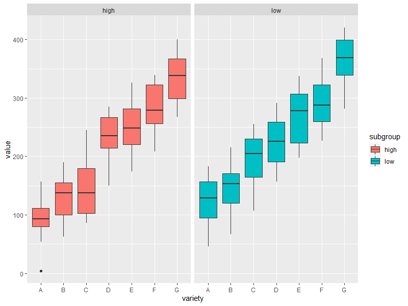
# Boxlot2
# One box per treatment
ggplot(data, aes(x=variety, y=value, fill=subgroup)) +
geom_boxplot() +
facet_wrap(~subgroup)
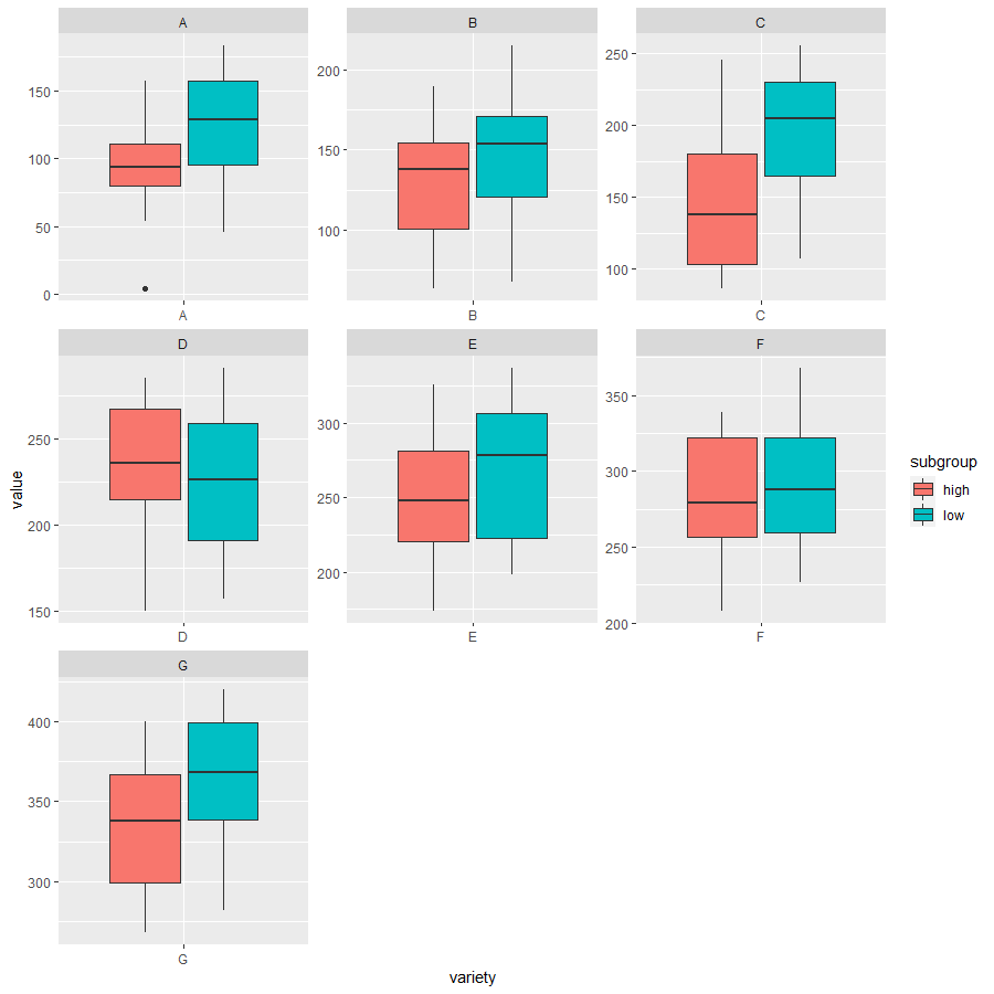
# Boxplot3
# one box per variety
ggplot(data, aes(x=variety, y=value, fill=subgroup)) +
geom_boxplot() +
facet_wrap(~variety, scale="free")

# Stacked bar plot
# library
library(ggplot2)
library(viridis)
library(hrbrthemes)

# create a dataset
specie <- c(rep("sorgho" , 3) , rep("poacee" , 3) , rep("banana" , 3) , rep("triticum" , 3) )
condition <- rep(c("normal" , "stress" , "Nitrogen") , 4)
value <- abs(rnorm(12 , 0 , 15))
data <- data.frame(specie,condition,value)

# Small multiple
ggplot(data, aes(fill=condition, y=value, x=specie)) +
    geom_bar(position="stack", stat="identity") +
    scale_fill_viridis(discrete = T) +
    ggtitle("4 Species Production under different environment") +
    theme_ipsum() +
    xlab("")

# Scatter plot with histogram
library(ggplot2)
library(ggExtra)

# classic plot :
p <- ggplot(mtcars, aes(x=wt, y=mpg, color=cyl, size=cyl)) +
      geom_point() +
      theme(legend.position="none")


# with marginal histogram
ggMarginal(p, type="histogram")

# Bubble plot
# Libraries
library(ggplot2)
library(dplyr)

# The dataset is provided in the gapminder library
library(gapminder)
data <- gapminder %>% filter(year=="2007") %>% dplyr::select(-year)

# Most basic bubble plot
data %>%
  arrange(desc(pop)) %>%
  mutate(country = factor(country, country)) %>%
  ggplot(aes(x=gdpPercap, y=lifeExp, size=pop, color=continent)) +
    geom_point(alpha=0.5) +
    scale_size(range = c(.1, 24), name="Population (M)")

# Doughtnut
# load library
library(ggplot2)

# Create test data.
data <- data.frame(
  category=c("A", "B", "C"),
  count=c(10, 60, 30)
)

# Compute percentages
data$fraction <- data$count / sum(data$count)

# Compute the cumulative percentages (top of each rectangle)
data$ymax <- cumsum(data$fraction)

# Compute the bottom of each rectangle
data$ymin <- c(0, head(data$ymax, n=-1))

# Compute label position
data$labelPosition <- (data$ymax + data$ymin) / 2

# Compute a good label
data$label <- paste0(data$category, "\n value: ", data$count)

# Make the plot
ggplot(data, aes(ymax=ymax, ymin=ymin, xmax=4, xmin=3, fill=category)) +
  geom_rect() +
  geom_text( x=2, aes(y=labelPosition, label=label, color=category), size=6) + # x here controls label position (inner / outer)
  scale_fill_brewer(palette=3) +
  scale_color_brewer(palette=3) +
  coord_polar(theta="y") +
  xlim(c(-1, 4)) +
  theme_void() +
  theme(legend.position = "none")

Advanced Graphs
Also, there are more advanced graphs could be created with R studio including some interactive plots. Those informative graphs enable us to deeper exploration of datasets.
Firstly, here are two examples of (interactive) treemap and circular bar plot. Both graphs demonstrate the partition of groups and subgroups in the dataset. However, treemaps underline the hierarchy relationships between groups and subgroups while circular bar plot focus more on the proportion of subgroups. Besides, treemaps are more appropriate when the number of groups is small and the size of group is big, but circular bar plot do the oppsite.
# Interactive Treemap
# library
library(treemap)
library(d3treeR)

# dataset
group <- c(rep("group-1",4),rep("group-2",2),rep("group-3",3))
subgroup <- paste("subgroup" , c(1,2,3,4,1,2,1,2,3), sep="-")
value <- c(13,5,22,12,11,7,3,1,23)
data <- data.frame(group,subgroup,value)

# basic treemap
p <- treemap(data,
            index=c("group","subgroup"),
            vSize="value",
            type="index",
            palette = "Set2",
            bg.labels=c("white"),
            align.labels=list(
              c("center", "center"),
              c("right", "bottom")
            )
          )

# make it interactive ("rootname" becomes the title of the plot):
inter <- d3tree2( p ,  rootname = "General" )
# Circular barplot
# library
library(tidyverse)
library(viridis)

# Create dataset
data <- data.frame(
  individual=paste( "Mister ", seq(1,60), sep=""),
  group=c( rep('A', 10), rep('B', 30), rep('C', 14), rep('D', 6)) ,
  value1=sample( seq(10,100), 60, replace=T),
  value2=sample( seq(10,100), 60, replace=T),
  value3=sample( seq(10,100), 60, replace=T)
)

# Transform data in a tidy format (long format)
data <- data %>% gather(key = "observation", value="value", -c(1,2))

# Set a number of 'empty bar' to add at the end of each group
empty_bar <- 2
nObsType <- nlevels(as.factor(data$observation))
to_add <- data.frame( matrix(NA, empty_bar*nlevels(data$group)*nObsType, ncol(data)) )
colnames(to_add) <- colnames(data)
to_add$group <- rep(levels(data$group), each=empty_bar*nObsType )
data <- rbind(data, to_add)
data <- data %>% arrange(group, individual)
data$id <- rep( seq(1, nrow(data)/nObsType) , each=nObsType)

# Get the name and the y position of each label
label_data <- data %>% group_by(id, individual) %>% summarize(tot=sum(value))
number_of_bar <- nrow(label_data)
angle <- 90 - 360 * (label_data$id-0.5) /number_of_bar     # I substract 0.5 because the letter must have the angle of the center of the bars. Not extreme right(1) or extreme left (0)
label_data$hjust <- ifelse( angle < -90, 1, 0)
label_data$angle <- ifelse(angle < -90, angle+180, angle)

# prepare a data frame for base lines
base_data <- data %>%
  group_by(group) %>%
  summarize(start=min(id), end=max(id) - empty_bar) %>%
  rowwise() %>%
  mutate(title=mean(c(start, end)))

# prepare a data frame for grid (scales)
grid_data <- base_data
grid_data$end <- grid_data$end[ c( nrow(grid_data), 1:nrow(grid_data)-1)] + 1
grid_data$start <- grid_data$start - 1
grid_data <- grid_data[-1,]

# Make the plot
ggplot(data) +

  # Add the stacked bar
  geom_bar(aes(x=as.factor(id), y=value, fill=observation), stat="identity", alpha=0.5) +
  scale_fill_viridis(discrete=TRUE) +

  # Add a val=100/75/50/25 lines. I do it at the beginning to make sur barplots are OVER it.
  geom_segment(data=grid_data, aes(x = end, y = 0, xend = start, yend = 0), colour = "grey", alpha=1, size=0.3 , inherit.aes = FALSE ) +
  geom_segment(data=grid_data, aes(x = end, y = 50, xend = start, yend = 50), colour = "grey", alpha=1, size=0.3 , inherit.aes = FALSE ) +
  geom_segment(data=grid_data, aes(x = end, y = 100, xend = start, yend = 100), colour = "grey", alpha=1, size=0.3 , inherit.aes = FALSE ) +
  geom_segment(data=grid_data, aes(x = end, y = 150, xend = start, yend = 150), colour = "grey", alpha=1, size=0.3 , inherit.aes = FALSE ) +
  geom_segment(data=grid_data, aes(x = end, y = 200, xend = start, yend = 200), colour = "grey", alpha=1, size=0.3 , inherit.aes = FALSE ) +

  # Add text showing the value of each 100/75/50/25 lines
  ggplot2::annotate("text", x = rep(max(data$id),5), y = c(0, 50, 100, 150, 200), label = c("0", "50", "100", "150", "200") , color="grey", size=6 , angle=0, fontface="bold", hjust=1) +

  ylim(-150,max(label_data$tot, na.rm=T)) +
  theme_minimal() +
  theme(
    legend.position = "none",
    axis.text = element_blank(),
    axis.title = element_blank(),
    panel.grid = element_blank(),
    plot.margin = unit(rep(-1,4), "cm")
  ) +
  coord_polar()+

  # Add labels on top of each bar
  geom_text(data=label_data, aes(x=id, y=tot+10, label=individual, hjust=hjust), color="black",alpha=0.6, size=4, angle= label_data$angle, inherit.aes = FALSE ) +

  # Add base line information
  geom_segment(data=base_data, aes(x = start, y = -5, xend = end, yend = -5), colour = "black", alpha=0.8, size=0.6 , inherit.aes = FALSE )  +
  geom_text(data=base_data, aes(x = title, y = -18, label=group), hjust=c(1,1,0,0), colour = "black", alpha=0.8, size=4, fontface="bold", inherit.aes = FALSE)

In addition, following are three examples codes. These could generate directed connected graphes like network diagrams, (interactive) sankey diagrams and chord diagrams. Those digrams indicate the flow or connection relationships between a couple of groups. Among them, the network diagrams emphasize more on the connection and direction between nodes and the size of nodes is proportional to the size of group. Sankey diagrams and chord diagrams are more similar since both of them focus on the flow among groups. But Sankey diagrams usually illustrate those flow between two groups while chord diagrams could illustrate the flow among multiple groups.
# Network
# library
library(igraph)

# create data:
links=data.frame(
    source=c("A","A", "A", "A", "A","J", "B", "B", "C", "C", "D","I"),
    target=c("B","B", "C", "D", "J","A","E", "F", "G", "H", "I","I")
    )

# Turn it into igraph object
network <- graph_from_data_frame(d=links, directed=F)

# Count the number of degree for each node:
deg <- degree(network, mode="all")

# Plot
plot(network, vertex.size=deg*6, vertex.color=rgb(0.1,0.7,0.8,0.5) )

# Sankey
# Libraries
library(tidyverse)
library(viridis)
library(patchwork)
library(hrbrthemes)
library(circlize)

# Load dataset from github
data <- read.table("https://raw.githubusercontent.com/holtzy/data_to_viz/master/Example_dataset/13_AdjacencyDirectedWeighted.csv", header=TRUE)
# Package
library(networkD3)

# I need a long format
data_long <- data %>%
  rownames_to_column %>%
  gather(key = 'key', value = 'value', -rowname) %>%
  filter(value > 0)
colnames(data_long) <- c("source", "target", "value")
data_long$target <- paste(data_long$target, " ", sep="")

# From these flows we need to create a node data frame: it lists every entities involved in the flow
nodes <- data.frame(name=c(as.character(data_long$source), as.character(data_long$target)) %>% unique())

# With networkD3, connection must be provided using id, not using real name like in the links dataframe.. So we need to reformat it.
data_long$IDsource=match(data_long$source, nodes$name)-1
data_long$IDtarget=match(data_long$target, nodes$name)-1

# Make the Network
sankeyNetwork(Links = data_long, Nodes = nodes,
                     Source = "IDsource", Target = "IDtarget",
                     Value = "value", NodeID = "name",
                     sinksRight=FALSE, nodeWidth=40, fontSize=13, nodePadding=20)
# Chord digram
# Libraries
library(tidyverse)
library(viridis)
library(patchwork)
library(hrbrthemes)
library(circlize)
library(chorddiag)

# Load dataset from github
data <- read.table("https://raw.githubusercontent.com/holtzy/data_to_viz/master/Example_dataset/13_AdjacencyDirectedWeighted.csv", header=TRUE)

# short names
colnames(data) <- c("Africa", "East Asia", "Europe", "Latin Ame.",   "North Ame.",   "Oceania", "South Asia", "South East Asia", "Soviet Union", "West.Asia")
rownames(data) <- colnames(data)

# I need a long format
data_long <- data %>%
  rownames_to_column %>%
  gather(key = 'key', value = 'value', -rowname)

# parameters
circos.clear()
circos.par(start.degree = 90, gap.degree = 4, track.margin = c(-0.1, 0.1), points.overflow.warning = FALSE)
par(mar = rep(0, 4))

# color palette
mycolor <- viridis(10, alpha = 1, begin = 0, end = 1, option = "D")
mycolor <- mycolor[sample(1:10)]

# Base plot
chordDiagram(
  x = data_long,
  grid.col = mycolor,
  transparency = 0.25,
  directional = 1,
  direction.type = c("arrows", "diffHeight"),
  diffHeight  = -0.04,
  annotationTrack = "grid",
  annotationTrackHeight = c(0.05, 0.1),
  link.arr.type = "big.arrow",
  link.sort = TRUE,
  link.largest.ontop = TRUE)

# Add text and axis
circos.trackPlotRegion(
  track.index = 1,
  bg.border = NA,
  panel.fun = function(x, y) {

    xlim = get.cell.meta.data("xlim")
    sector.index = get.cell.meta.data("sector.index")

    # Add names to the sector.
    circos.text(
      x = mean(xlim),
      y = 3.2,
      labels = sector.index,
      facing = "bending",
      cex = 0.8
      )

    # Add graduation on axis
    circos.axis(
      h = "top",
      major.at = seq(from = 0, to = xlim[2], by = ifelse(test = xlim[2]>10, yes = 2, no = 1)),
      minor.ticks = 1,
      major.tick.percentage = 0.5,
      labels.niceFacing = FALSE)
  }
)

