

This blog post aims to generate forecasts of house property sales using Vector Autoregression (VAR) models. The dataset is downloaded from:
https://www.kaggle.com/htagholdings/property-sales?select=ma_lga_12345.csv
We utilize “ma_lga_12345.csv” dataset that contains data resampled using Median Price Moving Average (MA) in quarterly intervals. The data range from 30 September 2007 to 30 September 2019 at the time of download (8 July 2020). We focus on predicting the house price using VAR model. First, let’s look at the dataset:
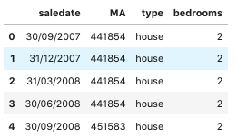
The dataset provides information on 2 types of property: house and unit. Each type of property is described with its MA price and number of bedrooms. Let’s forecast only the house prices first. We choose only “house” type and pivot the data so that we can feed it into the model as follows:

Figure 2 shows that there are 4 types of bedroom including bedroom 2, 3, 4 and 5. We realize that there are totally 4 missing values in bedroom 2 and bedroom 5 so we decide to exclude the first 2 observations from the dataset. The dataset after the pre-processing step can be summarized as follows:
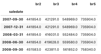
Figure 3 shows that there are 49 observations in total over time. Let’s look at the plot of house sale prices according to different number of bedrooms.

Figure 4 shows that there is an increasing trend over time in house prices in the first plot. The second plot called lag plot shows the observations at time 

An Autoregressive model is typically a linear of its own lags. In particular, the past values of the series are used to forecast the current and future values. Given the fact that we are dealing with multivariate time series data, VAR model is utilized as each variable in the VAR model is modeled as a linear combination of its past values and the past values of other variables in the system. Let’s suppose we have 2 variables 


where 


Similarly, we can increase the number of time series (variables) in the model which can make the system of equations become larger. As the VAR model requires the time series we want to forecast to be stationary, it is necessary to check whether all the time series in the system are stationary. We use ADF test to examine the null hypothesis (H0) that a unit root is present in time series sample, and the alternate hypothesis (H1) that the process has no unit root (is stationary). If p-value < 0.05 we reject that the data has a unit root (is non-stationary) in favor of H1.
Before applying VAR model to the dataset, we split data into training and test set. In addition, we use only the data of bedroom 2, 3 and 4 to train our model, the data of bedroom 5 is excluded from the training set. We utilize the data in the period from 2007 to 2017 to train our model, and use the two remaining year data to test our model. Thus, the training set includes 42 observations while the test set consists of 7 observations. We first taking logs of training set and use ADF to check all the series in training set for stationarity. Let’s look at the log-transformed house prices series in the training set as follows:

Figure 5 shows that each of the series has a fairly similar trend over the years except for the bedroom 2 whose different pattern is noticed after the 20th observation. Looking at the figure 5, we can be quite sure that the log-transformed series are not stationary as they show an increasing trend overtime. The p-value of ADF test for the log-transformed series confirms that the null-hypothesis, of non-stationarity, can not be rejected.
To transform the data to a working-stationary dataset, we first difference the data. We take the “first-order difference” – that is:

where 


After taking the first-order difference, all of the log-transformed series are still not stationary. So we take the second-order and third-order difference similarly, and all series are stationary after the third-order difference. To select the right order of VAR, we find the model with smallest AIC score. We can calculate a table of AIC score regarding different orders of VAR as follows:

Based on the results in Figure 6, we choose the selected order as 9 since the computed AIC is the lowest at lag 9. The VAR(9) model for 3 variables can be written by:

where 


After that, we train the VAR(9) model, and then get the results as follows:
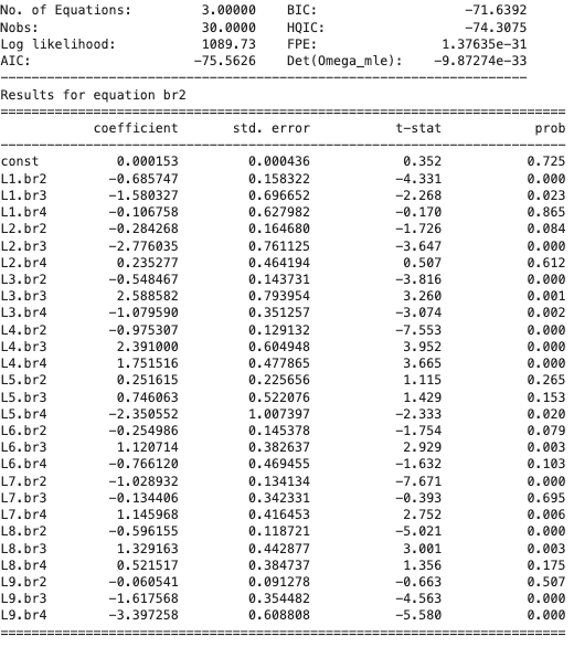
Figure 7 shows the results for equation of bedroom 2 which estimate the price of bedroom 2 in terms of past values of bedroom 2, 3, and 4 from lag 1 to lag 9. Equations of bedroom 3 and 4 also are similar to that of bedroom 2. After fitting the model, let’s look at the in-sample fit:

As can be seen from Figure 8, the yellow points (forecasted values) nearly fluctuate in the same manner as the blue stars (actual training values). As we take the third-order difference and use 9 lags to generate forecasts, there is no forecast for the first 12 observations.
Then, we generate one-step ahead static out-of-sample forecast (uses the actual previous value to compute the next one) and one-step ahead dynamic out-of-sample forecast (uses the previous forecasted value to compute the next one) for bedroom 2, 3, and 4. Out-of-sample forecasts for bedroom 5 is produced based on the fact that the bedroom 4 and 5 series have a fairly similar trend over the years, in addition, the price of bedroom 5 is nearly equal to the price of bedroom 4 multipled by 1.25 (See Figure 4). Thus, we generate out-of-sample forecasts for bedroom 5 based on the forecasted values of bedroom 4 multipled by 1.25.


Figure 9 shows that the VAR(9) generates fairly good one-step ahead static out-of-sample forecasts for the bedroom 2, 3, and 4 while it does not perform well for the bedroom 5. On the other hand, figure 10 shows that the VAR(9) performs well regarding one-step ahead dynamic out-of-sample forecasts for bedroom 3 while the model’s performance is still limited in terms of dynamic forecasts for bedroom 2, 4, and 5. From both figures, we can see clearly that static forecast is better than dynamic forecast.
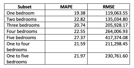
Let’s look at the forecast metrics including MAPE and RMSE:


Figure 11 shows that the bedroom 3 has the smallest values of MAPE and RMSE, followed by the bedroom 4 and 2 wheres the bedroom 5 has the largest values of MAPE and RMSE. In the mean time, Figure 12 shows that instead of the bedroom 5, the bedroom 2 has the largest values of MAPE and RMSE. In line with our analysis from Figure 9 and 10, Figure 11 and 12 show that static forecast gets smaller errors than dynamic forecast in general.
To generate the errors for all individual houses in the raw dataset, we regarded the forecasted values of individual houses in the same quarter as the forecasted values at the last day of this quarter generated by the VAR(9) using the median quarterly prices. For example, the forecasted value using the median quarterly prices on 31 March, 2018 is used as the forecasted value for all individual houses from 1 January, 2018 to 31 March, 2018. The training set ranging from 30 September 2007 to 31 December 2017 is used to generate one-step forecast for the test set including the two remaining year data. As the data set includes two types of property: house and unit, we generate forecasts for all individual units in a similar way. After doing that, we have the forecast errors for all individual houses and units as follows:

In summary, the VAR achieves quite good performance regarding the bedroom 1,2,3, and 4 whose data are used to estimate the model. Meanwhile, the VAR produces the worst forecasts for the bedroom 5 implying that using the forecasted values of bedroom 4 to estimate the values of bedroom 5 might be not an optimal approach. Moreover, static forecast achieves smaller errors than dynamic forecast in the MA data while there is not much difference between their errors in the raw data. One possible cause is that there are only 7 observations in test set of the MA data for each type of bedroom, and their forecasted values are used to imply forecasts for, for example, 1,664 observations of the house with bedroom 4 in test set of the raw data. Moreover, the actual price in the raw data fluctuates wildly. Therefore, the superiority of one-step ahead static forecast over one-step ahead dynamic forecast might been cancelled out in the raw data despite the fact that it performs much better than one-step ahead dynamic forecast in the MA data for both unit and house.
